1

Sea Level Rise in Australia and the Pacific

W. Mitchell, J. Chittleborough, B. Ronai and G.W. Lennon

Introduction

It is generally accepted that the determination of a trend in a sea level record is only possible when a long time series of observed elevations over many years is available. The small magnitude of the trend on the one hand, and the perturbation of the record by systematic noise over a wide range of frequencies on the other, determine that this is so. In the context of sea level trend analysis, the word ‘Noise’ can be considered to apply to any feature present in the observed record which impedes access to the underlying long term change of mean sea level. Prominent in this category, and especially in the tropical Pacific, are the sub-regional variations of sea level which occur in time scales of five to ten years and which are associated with the El Ni£o phenomenon. Such features, together with the notorious volcanic and tectonic crustal motions of the Pacific Rim affecting the land levels to which the observations are referred, are of particular concern to those who seek an early assessment of sea level trends in the region.

It is still too early to expect definitive estimates to be available from the South Pacific Sea Level and Climate Monitoring Project, but early indications, supported by occasional much longer miscellaneous time series from historic instrumentation might still be of interest. This suggestion is made despite the fact that the former high resolution series are of short duration, while the latter were invariably matched to less demanding specifications than is required for the resolution of the small trends of global warming. At the very worst, such an exercise offers opportunities in planning and defining interpretive procedures, together with assisting our understanding of the scale of the signal. In this manner, even at this early stage, such a process may be instrumental in setting bounds of acceptability to the output of the climate models which, in the nineteen eighties, raised the scares of inundation in the atoll nations.

Then it is not unreasonable that the study would have the potential to increase understanding of the scale of the signal to noise ratio in regions which have not yet figured prominently in the treatment of sea level trends. Also, some insight may be gained as to the relative contributions of sea level rise compared with land motion. In the latter context mutual benefit may be gained from the parallel study of sea level observations on the coastal fringe of the relatively stable Australian continental block, compared with the Pacific Islands which can be disturbed by tectonic, volcanic or biological (Coralline) motions.

At best then some light may be thrown upon the degree of spatial coherency, the importance of which must not be under-estimated. Large scale spatial coherency, for example, argues for reality and perhaps for the dominance of thermal influences on the surface layers of the ocean, rather than the addition of mass from melting land-based ice with consequent warping of the sea bed under load. It is suggested that the scale of Australasia and the Pacific Ocean qualifies for such consideration. Then there is the residual conundrum if coherency is poor.

Inadequate data, seabed warping under load and dominance of crustal motion may all play a part. In the latter circumstances it is still possible to proceed a little further on the understanding that we may expect that the climate change component is generally positive, in that the fact that sea levels are rising is generally agreed. In contrast a first premise may be accepted that the forces which determine land motion are more likely to produce motion in both vertical directions. Although not strictly true, given for example, the tendency for coastal structures, including tide gauge installations to be subject to subsidence, nevertheless there is a measure of truth in the premise.

In consequence then, if the sea level records are treated for a number of locations and the overall mean is taken of the several independent determinations of trends, then this mean has a tendency to provide greater focus on the trend of the world ocean, by reducing the effect of the more random land motions. In fact the assessments of the Intergovernmental Panel on Climate Change (IPCC) have adopted this premise. It may be possible also, proceeding further along these lines, to infer that sub-regional coherency may be an indicator of oceanic circulation at work. However such principles need to be exposed to practical examples and this is the aim of the present exercise. In a rigorous treatment of those observed series which happen to be available, and using new techniques of analysis designed specially for the treatment of trends in tidal time series, an attempt is made to evaluate the trends of sea

2

levels in the Pacific and in Australian coastal waters, with further reference to selected stations for which especially long time series of observed sea level are available.

Trends in Pacific Sea Level Records

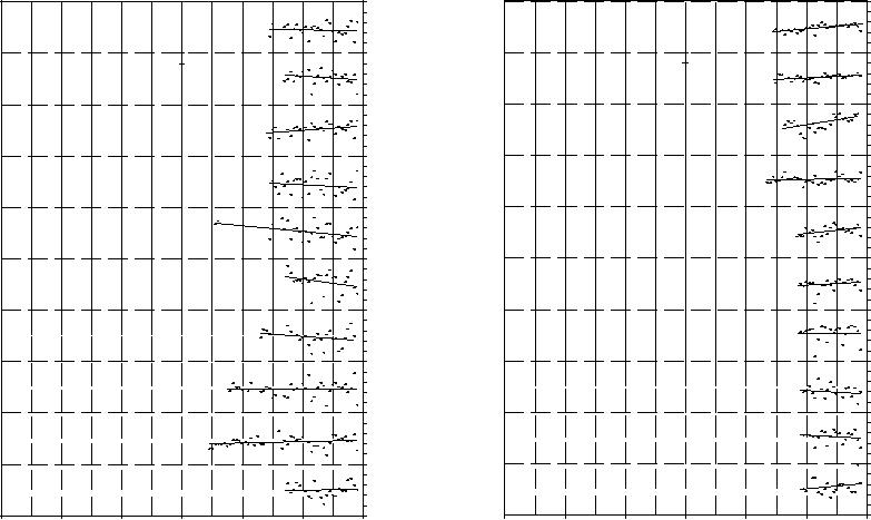
Conventional tide gauges have been operating in the South Pacific for several decades. Figure 1 (a-d) shows the annual mean levels and trends for the longer term observed records (each of more than 20 years of hourly values) held by the WOCE (World Ocean Circulation Experiment) Data Center at the University of Hawaii. There are forty individual records which fit into this category. The accompanying Table 1 lists the trends indicated by the analysis of those stations of this group which boast a record length covering 25 years or more.

The hourly values were analysed for 112 tidal constituents plus a trend term, using harmonic analysis over the entire dataset for each location. For some stations (Pohnpei, Yap. Christmas, Kanton, Papeete, Valpariso and Callao) there was also a function included in the treatment designed to identify any datum shift which might be contained in the record, and to make an appropriate correction so as to maintain datum stability in those cases where instrumental performance or its maintenance fell short of requirements. The resultant trend estimates are scattered, but lie within the range -11.5 mm per year at Kodiak Island, Alaska, and +5.5 mm per year at Chichijima, Japan. It is appropriate to assume that in these locations, it is the vertical land movement which contributes to their extreme results although the identification of the two separate components (land motion and sea level rise) is not otherwise possible. For this reason it is common to add the qualification of “relative” to the trend, ie. relative trend of sea level with respect to land levels. Again, ideally there is a clear need to ascertain the contribution to sea level trends of the motion of the land by independent means, perhaps by tracking such motion within a geodetic frame, utilising the latest features of satellite technology such as continuous high resolution (dual frequency) GPS (Global Positioning System).

The outstanding feature of Figure 1 is that the conventional tide gauge records for the Pacific are poor, with suspected datum shifts and large gaps in continuity. The indication is that there has been a rather haphazard approach to gathering sea level information in the region. The quality of the records suffers from a lack of coordination and a lack of attention to gauge maintenance. This is probably due to a focus that primarily captures sea level fluctuations rather than the sea level trends, and this is to be expected in that shorter term variations were the main issue and the initial target, rather than the long term sea level trend itself.

Nevertheless, the long term conventional tide gauge records show some coherency due to large scale oceanographic features such as the El Ni£o. In particular, the records show the influence of the El Ni£o events of 1982/3, 1987/8 and 1997/8 in the form of large negative departures from the run of mean sea level values. These excursions dominate the records from the affected gauges and will contribute substantially to the noise in the estimates of sea level trends at these locations. It is to be expected that the gauges located close to the equatorial wave guides, and in particular those near to the western boundary of the Pacific will undergo substantial fluctuations during these episodes. Here it is not uncommon that major positive shifts in mean sea level in response to sub-regional warm (and consequently low density) patches of ocean are typically of 30 to 40 cm, and these anomalies may persist for several months. It is for this reason and others, that it is scientifically unreasonable to consider historic records less than several decades to yield realistic estimates of sea level trends.

Taking the records from those stations which have data for more than 50 years (five stations in all – see Table1) and calculating the average trend over this period, one arrives at a figure of positive relative sea level rise of 1.07 mm per year. For stations that have data over periods greater than 25 years, and by this means broadening the base to 27 stations listed in Table 1, the figure for the mean trend is positive again but has been reduced to 0.8 mm per year. Note from the above remarks that the broadening of the base carries the prospect of some reduction of the contribution from land motion and a closer focus on that part of the trend which depends upon climate change. This result is on the low side of the IPCC estimate of 1995 (IPCC, 1995) which suggests that the global trend lies between 1 and 2 mm per year. The same observed data used here in Figure 1 and Table 1 were included in the estimates published by the IPCC, although it should be noted that the latter were based upon a much larger world-wide base. Also analytical procedures adopted here represent a new development which we believe are better matched to the specific problem of sea level trend analysis. Again, the indication

3

might be that in other parts of the global oceans, there are many gauges which show trend rates greater than those of the Pacific. Another explanation of the differences could be that the contributions from vertical land motion were somewhat greater in the stations used by the IPCC and also that the land motion had a positive bias.

In referring to the indications of Figure 1 and Table 1, the following comment is appropriate. Allowing for the expected presence and nature of the noise level which contributes variability to the sea level record from year to year, the data series in each case lends itself to fitment by a linear trend. It would only be in the case of certain longer time series that an attempt may be made to search for changes in trend with time. It will be acknowledged, nevertheless that visually at least, and at this stage, there is no clear evidence for an acceleration in sea level trends over the course of the last century. Personnel familiar with sea level work were cautious to accept the findings of the early numerical climate models, which triggered much of the anxiety among coastal dwellers over the last two decades. These models forecast rapidly accelerating sea level trends. The hard facts of sea level observations identified here, serve to confirm a more moderate view of sea level trends..

Location	Years of data	Estimated Trend
		(mm per year)
Majuro	27.9	+2.19
Malakal	28.2	-1.34
Rabaul	26.9	-2.21
Rikitea	27.0	+1.28
Noumea	31.6	-0.40
Midway	48.6	+0.00
Wake	44.9	+1.81
Johnston	50.1	+0.72
Guam	47.7	-0.37
Chuuk	27.6	+1.79
Kwajalein	51.8	+0.81
Pago Pago	42.4	+1.43
Honolulu	92.8	+1.51
Nawiliwili	44.0	+1.48
Kahului	44.7	+2.14
Hilo	57.5	+3.39
Mokuoloe	31.6	+1.16
Antofagasta	51.0	-1.07
Buenaventura	41.3	+2.74
Quepos	28.4	+0.41
Callao	40.0	+0.83
Pohnpei	25.9	-0.69
Yap	28.9	-2.72
Christmas	38.3	+0.00
Kanton	43.0	+0.71
Papeete	29.3	+2.51
Valparaiso	47.1	+2.75

Table 1: The estimated relative sea level trends for tide gauge locations in the Pacific region from the University of Hawaii archive which have at least 25 years of hourly data The overall average relative sea level trend in the above list is +0.77 mm per year.

4

Trends in Australian Sea Level Records

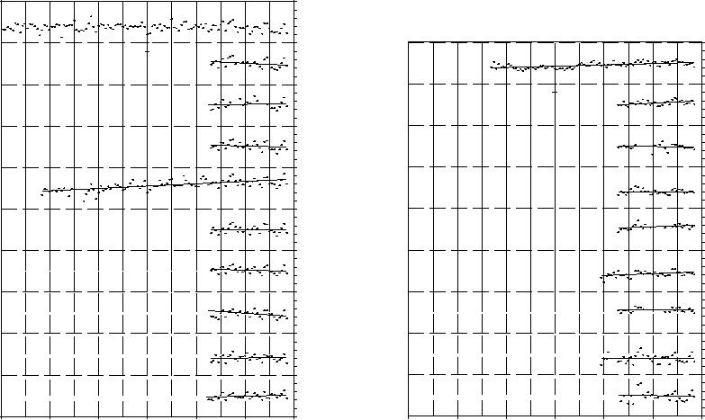
A similar analytical process has been applied to the output of the conventional sea level gauges installed along the coastline of Australia. By “conventional”, the implication is that the instrumentation is of some vintage so that long records are available, but that its specifications tend to target port operations rather than scientific study. As in the earlier Pacific case, the plots of annual means and their trends are presented in Figure 2 (a-c) for those stations which had achieved a record of at least 25 years of hourly data. Trend rates are given in Table 2. Again, taking the average of the group, the indication is that Australian relative sea level trends show +0.3 mm per year, substantially less than the IPCC estimate and also less than was found for the Pacific case.

In understanding this perhaps surprising result, the importance of supplementary information is underlined. If an attempt were to be made to translate the findings into absolute, as opposed to relative sea level rise, it would be necessary to take into account the vertical land movements at the tide gauge sites. Indeed, one may see that for Port Adelaide Inner and Outer, there is quite a large positive rate of relative sea level rise, while for Port Pirie, located further north along the Adelaide geosyncline, there is a small negative rate. The Port Adelaide sites have been studied intensively and a paper explaining the larger than expected positive trend here has been written by Belperio, 1997. He explains the rate by local land subsidence due to the construction of levees and the withdrawal of groundwater since European settlement. The geodesists suggest that the reason for the north-south tilting along the geosyncline may be partly due to post-glacial rebound and is described in a paper by Harvey et al, 1998.

A striking feature of the plots is the degree of correlation in the shorter term fluctuations of the annual values, considered anticlockwise around the coast from Darwin in the north to Victor Harbor south of Adelaide, although there exists a small measure of visual correlation to be seen further to the east in the Bass Strait sites listed in the lower half of Figure 2c. It is significant that the correlation between the sites from Darwin around the west and south of the continent, is reflected in the Southern Oscillation Index (SOI) which is plotted for convenience at the head of Figure 2a. Of course the SOI is an indicator of large scale atmospheric variation in the Pacific associated with the El Ni£o phenomenon. For example the SOI declined significantly in the period of 1988 to 1994, then rose sharply to a peak in 1996 with a sharp reversal in 1997 due to a strong positive El Ni£o event. In the same interval, sea levels dropped from 1988 onwards, but only until 1993. when they began to reverse, to reach a peak in 1996 to be followed by a sharp decline in 1997. The links are clear, and this spatial coherence argues for variability in the sea level record that is real, and certainly not noise from instrumental imperfections. The variability is clearly a signal that has its source in major features of ocean/atmosphere interaction. Over periods of five to ten years such fluctuations are prone to occur, and for such periods they superimpose upon the small background trend in sea levels, excursions of the mean over several centimetres.

Yet another feature of interest in the plots is the decline in sea levels at Port Pirie in the 1930s followed by an equally long period of recovery in the 1940s. This feature most likely is an indicator of yet another real mechanism, perhaps a large scale oceanographic feature, but perhaps also, given the unique location of the station, this might be due to a feature arising from gulf processes. Port Pirie is located in Gulf St Vincent which is known to have difficulty in its annual refreshment by the release of salt which accumulates due to an excess of evaporation over precipitation in the upper reaches of that Gulf. It is just possible that climate variation may lead to inadequate refreshment over a number of years so that higher salinities, and therefore resident water which is of higher density than is the norm, may have been allowed to accumulate over a number of years leading to lower Gulf water levels.

Perhaps South Australia is a little unusual since a body of supplementary evidence is available to help understand the variability of the record. The experience does however underline the fact that the task of interpretation of a long term trend from an observed sea level series, is complex and perhaps the only solution to the problem is to eliminate whatever noise is possible to eliminate and then study the continuing long time series to allow time to cure the shorter term confusion. For example it is known that there exists a very small tidal wave which has a period of 18.61 years, ie. a single wave which requires 9.3 years to rise from its trough to its peak and a further 9.3 years to complete the cycle falling back to the trough. This is due to the precession westwards of the node of the orbit of the Moon (the point where the orbit crosses the Ecliptic). In this survey, this tide has been included in the calculations.

5

Meanwhile the trends identified in the present work will, no doubt, be refined as further data is accumulated.

The important questions remain. Firstly what advantage will be seen when the data series from the higher resolution generation of instruments become long enough to be subjected to exhaustive analysis? There is confidence that a considerable improvement will be seen when the SEAFRAME stations reach their maturity for example. Secondly, to what extent is there developing an understanding of a minimum length of data series capable of providing useful information on sea level trends? Is it possible to answer the question; “How long is long enough?” What follows addresses just such questions.

Location	Years of data	Estimated Trend
		(mm per year)
Darwin	34.9	-0.02
Wyndham	26.4	-0.59
Port Hedland	27.7	-1.32
Geraldton	31.5	-0.95
Fremantle	90.6	+1.38
Bunbury	30.2	+0.04
Albany	31.2	-0.86
Esperance	31.2	-0.45
Thevenard	31.0	+0.02
Port Lincoln	32.3	+0.63
Port Pirie	63.2	-0.19
Port Adelaide – Inner	41.0	+2.06
Port Adelaide – Outer	55.1	+2.08
Victor Harbor	30.8	+0.47
Hobart	29.3	+0.58
Georgetown	28.8	+0.30
Williamstown	31.8	+0.26
Geelong	25.0	+0.97
Point Lonsdale	34.4	-0.63
Fort Denison	81.8	+0.86
Newcastle	31.6	+1.18
Bundaberg	30.2	-0.03
Townsville	38.3	+1.12

Table 2: The estimated relative sea level trends for tide gauge locations around Australia which have at least 25 years of hourly data on the National Tidal Facility archive. The overall average relative sea level trend in the above list is +0.30 mm per year.

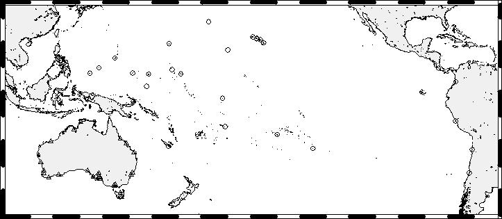
Figure 3, and the accompanying index, identify the locations of the stations for which trends are listed in Tables 1 and 2.

Asymptotic Trend Evaluation

The estimate of trends in sea level data has been fraught with difficulties due to inadequate quality control of the gauges themselves, datum shifts and combinations of oceanographic and meteorological influences over various time scales. As indicated above in the case of Port Pirie, there are oceanographic perturbations of sea level over twenty years and even longer. The question then arises as to how long is an appropriate length of sea level data to determine unmistakably the background or secular sea level trend?

In a search for an answer to this important question, which lies in the background of all research into trends, the NTF has proceeded on an empirical basis by conducting experimental analytical processes on the few existing long period datasets. Some of the longest data series available have been collected for San Francisco, Honolulu, Fremantle, Fort Denison (Sydney), Port Pirie and Port Adelaide, three of

6

these being Australian locations of which two are South Australian. These five datasets form the basis of the study.

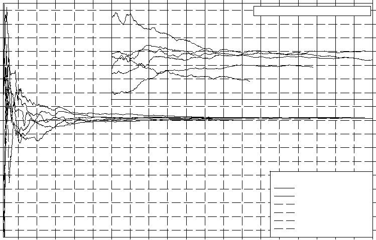
To begin the analysis, the first year of observed hourly values of sea level for the first location was analysed for a trend. The full harmonic model of 112 tidal constituents was applied so as to identify the tidal component and at the same time a trend analysis is conducted. The value of this trend is then plotted at the origin of Figure 4. The next stage begins by adding just one month of additional hourly data, repeating the analysis and plotting the trend result in Figure 4. The process is repeated adding one month at a time to the dataset presented for analysis until the entire available dataset is exhausted. Each estimate given and plotted then is the sea level trend evaluated over the entire preceding time series, regardless of the start date for a particular station.

The resultant plot demonstrates that the initial estimates of trend are understandably noisy, given that the series are quite short and subject to significant perturbation. The latter arise from two major sources. Firstly the addition of individual months to a short time series presented for analysis results in small changes in the estimates of the tidal amplitudes and phases. Secondly, the products of ocean/atmosphere interaction, and the like, perturb the trends significantly in the early stages until the use of long time spans acts to minimise their effects. As the length of the data sets grow, the additional month of data is progressively less likely to change the trend estimate, leaving a relatively smooth time series of trend estimates. Figure 4 suggests that by the time thirty years (360 months) has been processed, the estimates are reasonably reliable, but one may still see adjustments occurring out to fifty years (600 months).

There is strong evidence in this figure that the final rates are not the same at all locations. San Francisco can be said to show a slight upward trend in the plot that could be claimed as corresponding to a small acceleration in sea level rise. The opposite is true for Fremantle. Port Pirie quite clearly also shows a deceleration in relative sea level trends, which may be explained by a rise in the land upon which the gauge is operating (note the previous discussion of the Port Pirie anomaly). A similar deceleration is shown for Adelaide and the probable influence of tilting in the Adelaide geosyncline has already been discussed. Honolulu is an interesting case in view of its oceanic exposure, and as may be expected at this station, the early discrepancies are somewhat less than the other stations. Nevertheless small adjustments appear in both directions as time elapses, even as the full century of observation approaches, but here again, there is no clear evidence of acceleration of the trend.

It can be shown that the rate of sea level rise at Fremantle has decreased by 1mm per year over the last fifty years with a current estimate of +1.38mm per year (as already listed in Table 2). Note should be taken here that Fremantle is a location where the tidal range (Highest to Lowest Astronomical Tide) is a mere 1.2 metres so that meteorological effects, rather than tidal effects, dominate the record. The rate at Fort Denison has remained remarkably steady over the last 40 years. This is in contrast with the IPCC assessment that sea level rates are set to increase by two to six times over the next 100 years. The acceleration assessment from worldwide industrialisation over the last two centuries seems to be very slow to appear. What can be said is that accelerations of the trends identified in this exercise, are at best extremely small, at least on this evidence from just five available long datasets. Further studies of this type are necessary in order to broaden discussion on these and associated aspects of the sea level rise issue, and this is planned.

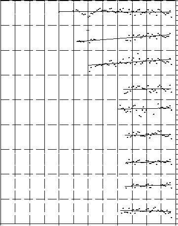
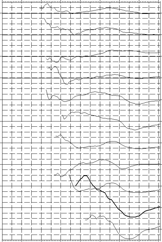
Sea Level Trends from the SEAFRAME gauges

In the light of the above analysis of the length of time necessary to determine accurate rates of relative sea level rise, it is premature to consider that the current high resolution South Pacific Sea Level and Climate Monitoring Project can provide anything other than “noisy” estimates of the trends. It is still true however, that the high resolution and accuracy of the new tide gauge technology will allow the secular trends to be determined in the shortest possible time scale.

To obtain at least some indication of the time taken for the estimates to asymptotically approach the secular trend, we have analysed the six minute sea level data from the South West Pacific in the same way as above and present the results in Figure 5. This demonstrates the large influences that the recent El Ni£o and La Ni£a events have had on the estimates of the trends, since for 6 of the 11 stations, the rates are an order of magnitude greater (positive and negative) than we would expect. We do see

7

however, that the estimates are becoming progressively smaller in magnitude and that the lines are becoming smoother.

The actual values of the trend, estimated from the observed data, are still worthy of consideration for other reasons. Problems arise, as in most countries, which affect individuals and their livelihoods. In many Pacific Islands, such concerns are overlain by the additional exposure to sea level rise because of their low topography. Nevertheless other problems of human activity remain, as elsewhere in the world. It becomes important then to ascertain whether a recent crop loss, or localised erosion episode is due to a short term natural event such as a storm surge or tropical cyclone, or indeed a seismic event, or even due to pollution or other human activity. Identification may lead to an assessment of the potential frequency of repetition, so that rectification strategies may be planned. In certain cases a rapid change to human practice and activity may be recommended. Other cases, particularly those associated with global warming, may imply long term adaptation measures. The sea level record will help considerably in defining the cause and nature of the perceived threat by defining time and height scales to be compared with the long term trend.

The following table quantifies the approximate changes in sea level at the sites of the new gauges since their installation.

Location	Number of years	Sea level change (cm)
Fiji	7.3	+1.01
Vanuatu	6.2	+0.92
Tonga	7.0	+13.34
Cook Islands	6.9	+4.83
Samoa	6.9	-3.22
Kiribati	6.8	-11.74
Marshall Islands	6.3	+1.98
Tuvalu	6.8	-8.69
Nauru	6.5	-10.82
Solomon Islands	5.3	+2.87
Papua New Guinea	4.2	+5.96

Table 3: Length of record and indicated sea level change for the SEAFRAME stations of the South Pacific Sea Level and Climate Monitoring Project

The listed values show that for stations in Kiribati, Tuvalu and Nauru there have been significant sea level falls since the start of the project, and that stations in Tonga and Papua New Guinea have shown a sea level rise. It is expected that as the effects from the recent El Ni£o and La Ni£a events subside, these locations will also register much lower rates of sea level change.

Conclusions

We have examined the long term rates of sea level change as registered on tide gauges in the Pacific region and found that it is difficult to estimate localised rates of change. Taking the 27 longest records available, the estimated mean relative sea level rise emerges as +0.8 mm/yr. This is on the low side of the global rate published in the IPCC Scientific Assessment.

We have also examined the records from the conventional tide gauges in the Australian coast zone. The estimated average rate of sea level rise from the longest records is computed to be +0.3 mm/yr, almost an order of magnitude less than the IPCC estimates.

Although the strongest feature of the Asymptotic Trend Evaluation adopted here is to identify the linear trend over the total recorded time series, the plotted points which make up Figure 3 provide a computed trend for each station up to the date to which the point refers. Consequently the later plots are affected by any recent change in the trend which may be present. This being so, it is relevant to comment that in both the above-mentioned data sets, it is difficult to find evidence of any change in the sea level trend (acceleration) in the whole region, as might have been expected, based upon the output of the climate models. Consequently over a major part of the world ocean, which on the one hand includes ocean stations, and on the other a major continental coastline, the indication is that, over recorded

8

history, sea level rise has occurred, but at a rate which falls significantly short of the IPCC world assessment. The question then arises as to the general status of knowledge of ocean/atmosphere interaction. Is it possible, for example, that the indications of real sea level trends, which are derived from observations, may set tighter bounds on the prognoses of the numerical models?

The Asymptotic Trend Evaluation of some long term sea level records here, establishes the fact that it may take at least thirty years to estimate consistent trends based upon the output of conventional tide gauges. The influence of El Ni£o & La Ni£a phenomena are clear and demonstrate that for some countries, and especially for the tropical Pacific, there have been significant variations of level, both positive and negative, in time-scales of five to ten years throughout the record. Research into such variability will lead to a better understanding of the physics of these events. The prospect then will be to remove from the analysis, a significant part of the shorter term variability which inhibits an early estimate of the background trend. Meanwhile, geodetic research might focus upon vertical land motion, which represents the other major inhibiting factor. In fact it is not unrealistic to anticipate a situation in which an estimated extrapolation of land motion may be possible. Then, with the assistance of sea level gauges of the new technology installed in the West Pacific and the Australian region, which provide greater resolution and an improved ability to identify the component parts of the record, we may be assured that less time will be expended in achieving the required stability of the computed trend.

References

Belperio, A.P., 1993. Land subsidence and sea-level rise in the Port Adelaide estuary: implications for monitoring the greenhouse effect,. Australian Journal of Earth Sciences, 40, 359-368.

Harvey, N., Barnett, E.J., Bourman, R.P. and Belperio, A.P.,1999. Holocene sea-level changes at Port Pirie, South Australia. Implications for global sea-level rise, Journal of Coastal Research, 15, 3, 607- 615.

Intergovernmental Panel on Climate Change, 1995. Climate change 1995. The science of climate change. Changes in sea level. Chapter 7, 359-406. In:J.T. Houghton et al., (eds.). Contribution of WG1 to the Second Assessment Report of the Intergovernmental Panel on Climate Change, Great Britain, Cambridge University Press, 672p.

W. Mitchell is the Deputy Director of the NTF, J.Chittleborough and B Ronai are Research Scientists at the NTF, and Prof G.W.Lennon is Editor of the Newsletter at the NTF.

Figure 1(a-d): Relative sea level trend analysis for forty stations in the Pacific for which more than twenty years of hourly observations are available courtesy of the University of Hawaii archives. The trend line in each case is based upon an Asymptotic Trend Analysis, as described later in the text, and the plotted points represent the observed annual mean sea levels.

Figure 2(a-c): Relative sea level trend analysis for twenty-seven stations on the Australian coastline for which at least twenty-five of hourly observations are available, in the National Tidal Facility archives. The trend line in each case is based upon an Asymptotic Trend Evaluation, as described later in the text, and the plotted points represent the observed annual mean sea levels. For comparison purposes, Figure 2a also contains a plot of the Southern Oscillation Index

Figure 3: Map, with index, to identify the locations of the stations listed in Tables 1 and 2

Figure 4: The Asymptotic Trend Evaluation applied to six exceptionally long observed sea level time series. The plotted graphs are accumulated for each station from repetitive monthly least squares analyses, which compute and remove the tidal contribution to the observed record up to that date, using a harmonic model, and in the same computation extract the linear trend for the same epoch. The inset plots the same data with a ten times expansion of the trend scale, but ignoring the first 360 months (30 years) of the record.

9

Figure 5: Relative sea level trend analysis for the eleven SEAFRAME stations in the South Pacific Sea Level and Climate Monitoring Project based upon data acquired to date, identifies apparent sea level change in the period of the record.

SEA LEVEL TRENDS FROM LEAST SQUARES ANALYSES (mm/year)

SEA LEVEL TRENDS FROM LEAST SQUARES ANALYSES (mm/year)

Cabo San Lucas (Mexico)							Nawiliwili (USA)
1.93							1.48
Kodiac (Alaska)			10 cm				Honolulu(USA)			10 cm
-11.5							1.51
Chichijima (Japan)							Kahului (USA)
5.55							2.14
Midway (USA Trust)							Hilo (USA)
0.00							3.39
Wake (USA Trust)							Mokuoloe (USA)
1.81							1.16
Johnston (USA Trust)							Antofagasta (Chile)						11
0.72							-1.07
Guam (USA Trust)							Valparaiso (Chile)
-0.37							2.75
Chuuk (FSM)							Buenaventura (Colombia)
1.79							2.74
Kwajalein (Rep Marshall Is)							Quepos (Costa Rica)
0.81							0.41
Pago Pago (USA Trust)							Callao (Peru)
1.43							0.83
1880	1900	1920	1940	1960	1980	2000	1880	1900	1920	1940	1960	1980	2000
			Year							Year

Figure 1(c)

Figure 1(d)

SEA LEVEL TRENDS FROM LEAST SQUARES ANALYSES (mm/year)

Port Pirie -0.19

Inner Harbor	10 cm
2.06

Outer Harbor 2.08

Victor Harbor 0.47

Hobart 0.58

13

Georgetown 0.30

Williamstown 0.26

Geelong 0.97

Point Lonsdale -0.63

1880

1900

1920

1940

1960

1980

2000

Year

Figure 2(c)

	120˚						150˚				180˚			210˚	240˚	270˚	300˚
30˚											30						30˚
													38 37
											31		41	39
														40
												32
								33
						47			34	46	35 25						44
					26
										48							43
0˚																	0˚
									27			49
				1								36					45
				2
														50
		3						24
								23			29				28
																	42
									22
-30˚	4																-30˚
	5				9				21
						11											51
	6		8
		7		10		12,13											14
						1418		17
							19
								16
								15
	120˚						150˚				180˚			210˚	240˚	270˚	300˚

1	Darwin		14	Victor Harbor	27	Rabaul	40	Hilo
2 Wyndham			15 Hobart		28 Rikitea		41 Mokuoloe
3 Port Hedland			16 Georgetown		29 Noumea		42 Antofagasta
4	Geraldton		17	Williamstown	30	Midway	43	Buenaventura
5 Fremantle			18 Geelong		31 Wake		44 Quepos
6	Bunbury		19	Point Lonsdale	32	Johnston	45	Callao
7 Albany			20 Fort Denison		33 Guam		46 Pohnpei
8 Esperance			21 Newcastle		34 Chuuk		47 Yap
9	Thevenard		22	Bundaberg	35	Kwajalein	48	Christmas
10 Port Lincoln			23 Mackay		36 Pago Pago		49 Kanton
11		Port Pirie	24	Townsville	37	Honolulu	50	Papeete
12		Port Adelaide - Inner	25	Majuro	38	Nawiliwili	51	Valparaiso
13		Port Adelaide - Outer	26	Malakal	39	Kahului

								Asymptotic Trend Evaluation
	80					5								Inset: Trend axis expansion				Months axis overlay
	70					4
	60				Trend(mm/yr)	3
	50					2
	40					1
	30					0
	20					-1
Trend(mm/yr)	10
	0																					15
	-10
	-20
	-30
	-40														SERIES		GAUGE		START		END
	-50																Fremantle		1897		1996
																San Francisco			1901		1998
	-60																Honolulu		1905		1998
	-70																Fort Denison		1914		1997
																	Port Pirie		1930		1997
	-80															Port Adelaide			1940		1997
	60	120	180	240	300	360	420	480	540	600	660	720	780	840	900	960	1020	1080		1140		1200
										Months